This vignette demonstrates how to use the ffaframework
package to perform flood frequency analysis under the assumption of
nonstationarity (NS-FFA). Readers unfamiliar with stationary FFA
workflows should first consult the Stationary FFA vignette.
The framework supports three forms of nonstationarity, modeled as linear trends in the distribution parameters:
- A linear trend in the location parameter.
- A linear trend in the scale parameter.
- A linear trend in both the location and scale parameters.
The shape parameter is treated as a constant due to difficulties in estimation caused by sample size limitations.
Case Study
This vignette will explore data from the Bow River at Banff
(05BB001), a station in the Reference Hydrometric Basin Network. The
station is unregulated, which suggests that trends in annual maxima are
caused by changes in climate as opposed to changes in land use or cover.
Data for this station is provided as CAN-05BB001.csv in the
ffaframework package.
library(ffaframework)

df <- data_local("CAN-05BB001.csv")
head(df)
#>   year max
#> 1 1909 314
#> 2 1910 230
#> 3 1911 264
#> 4 1912 174
#> 5 1913 232
#> 6 1914 214

plot_ams_data(df$max, df$year, title = "Bow River at Banff (05BB001)")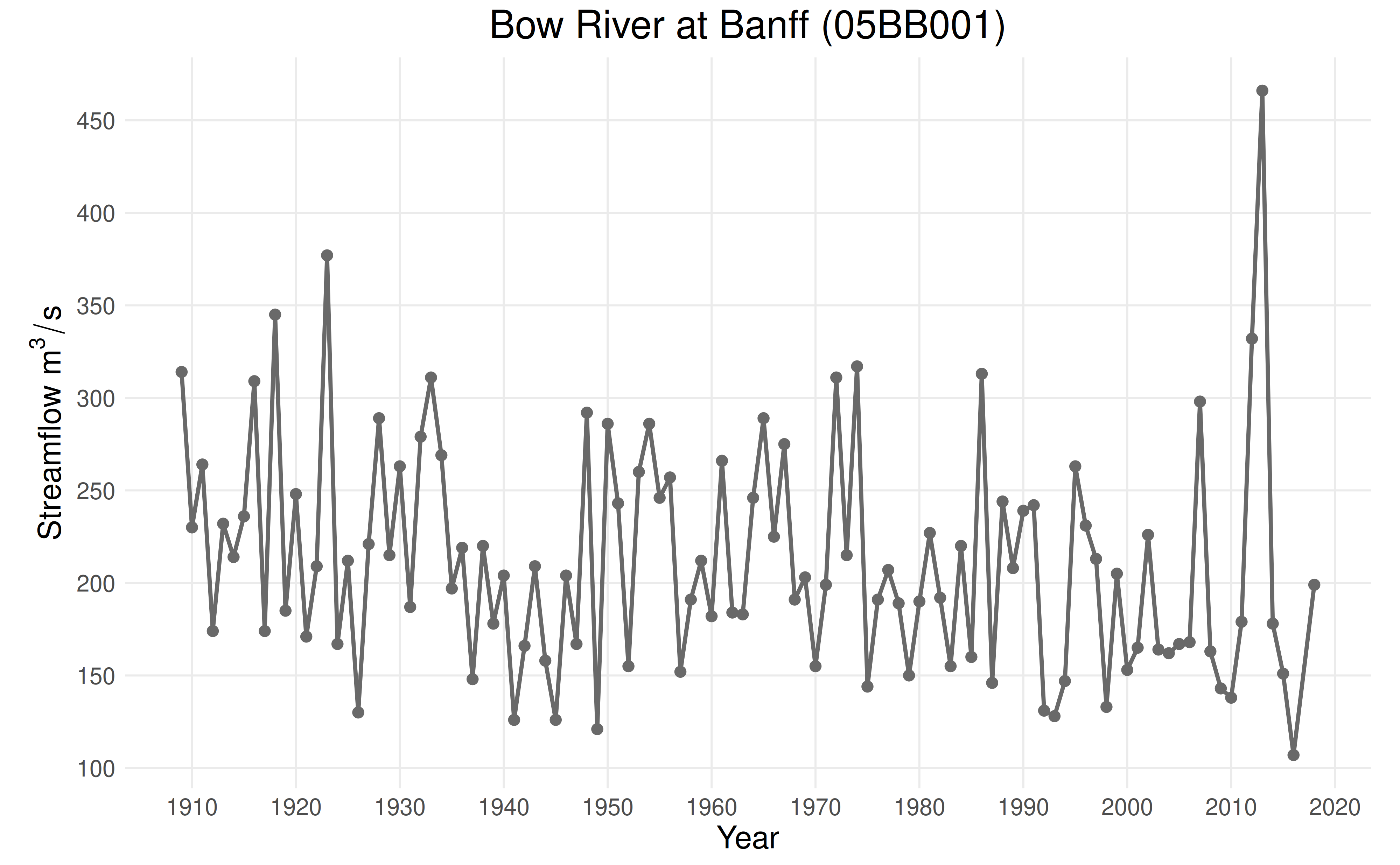
The ns_structure List
This vignette assumes a scenario where a trend in the mean has been
identified. To specify a trend in one or more distribution parameters,
create a ns_structure (nonstationary model structure) list
containing the boolean items location and
scale. Setting these items to TRUE adds a
trend to the location/scale parameter respectively.
ns_structure <- list(location = TRUE, scale = FALSE)Note: For guidance on trend detection, refer to the Trend Identification vignette.
Distribution Selection
L-moment-based distribution selection remains applicable under
nonstationarity, but requires dataset decomposition (detrending) prior
to analysis. The select_* methods do this automatically
(using the data_decomposition method) if the
ns_years and ns_structure arguments are
supplied.
selection <- select_ldistance(
    df$max,
    ns_years = df$year,
    ns_structure = ns_structure
)

print(selection$recommendation)
#> [1] "GNO"

plot_lmom_diagram(selection)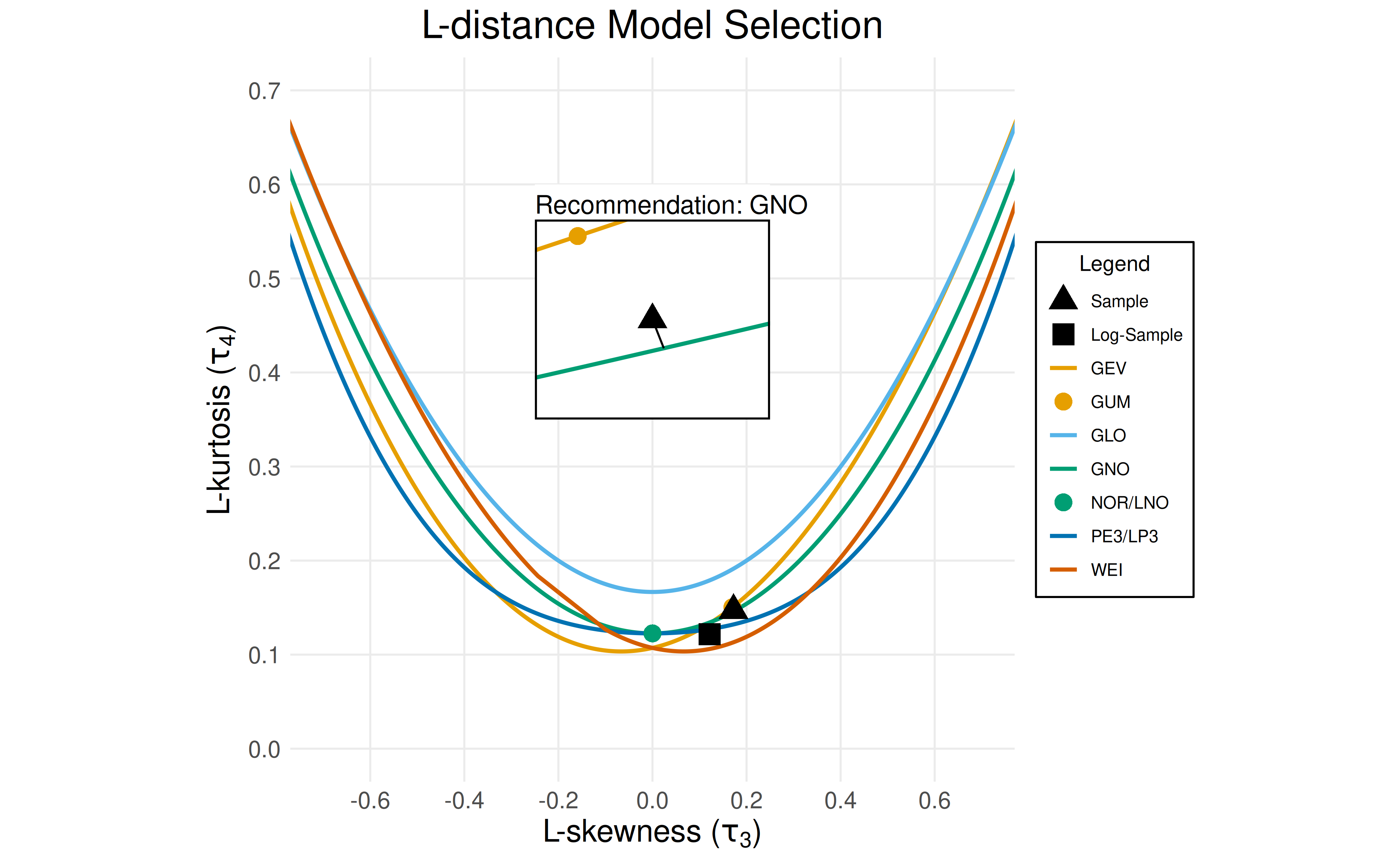
Note: The sample and log-sample points on the L-moment diagram are based on the detrended data.
Conclusion: The generalized normal (GNO) distribution is the best-fit distribution for the sample.
Parameter Estimation
Because L-moments parameter estimation requires stationarity, we will
use maximum likelihood estimation for this nonstationary model. The
fit_mle function implements maximum likelihood estimation
for both stationary and nonstationary distributions. It has two required
arguments:
-
data: The annual maximum series observations. -
model: A three-letter code corresponding to a probability distribution (ex."GNO").
Since a nonstationary model is used, two additional arguments are required:
-
ns_years: The corresponding vector of years for the observations indata. -
ns_structure: The nonstationarystructureobject described above.
fit <- fit_mle(
    df$max,
    "GNO",
    ns_years = df$year,
    ns_structure = ns_structure
)

print(fit$params)
#> [1] 224.0496619 -35.5153685  54.6324886  -0.3689085

print(fit$mll)
#> [1] -590.7329

plot_nsffa_fit(fit, slices = c(1915, 2015))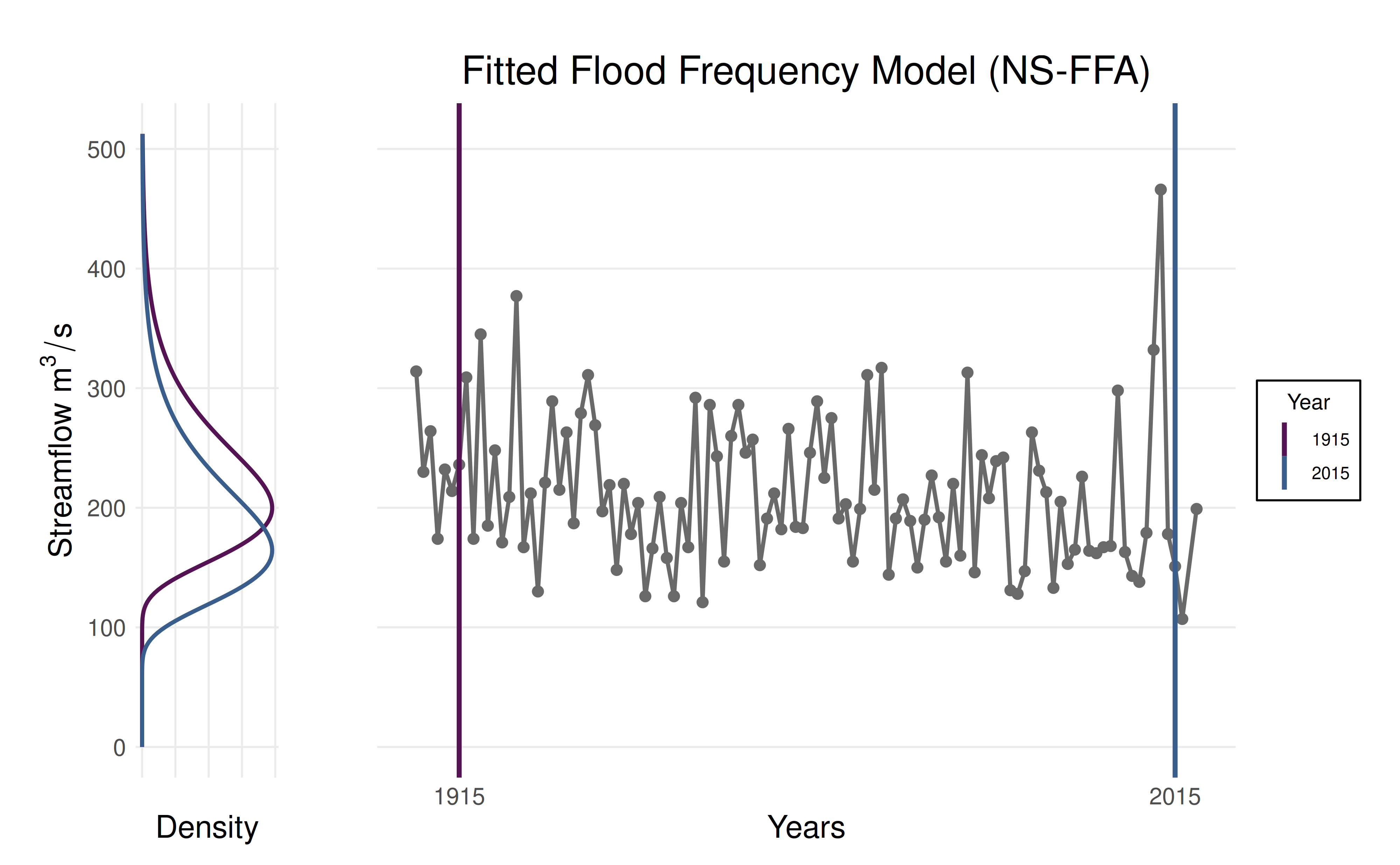
Note: The fitted parameters are: \((\mu_0, \mu_1, \sigma, \kappa)\), where the time-dependent location is modeled as \(\mu(t) = \mu_0 + \mu_1 t\). The covariate \(t\) is a linear function of the years: \((\text{years} - 1900) / 100\).
Uncertainty Quantification
Uncertainty quantification is an important step in NS-FFA as well as
S-FFA. In addition to the parametric bootstrap, the framework implements
the regula-falsi profile likelihood (RFPL) method for MLE. The
uncertainty_rfpl method has two required arguments:
-
data: The annual maximum series observations. -
model: A three-letter code corresponding to a probability distribution (ex."GNO").
Since our model has a nonstationary structure, three additional arguments are required:
-
ns_years: The corresponding vector of years for the observations indata. -
ns_structure: The nonstationarystructureobject described above. -
ns_slices: The years at which return levels are computed.
uncertainty <- uncertainty_rfpl(
    df$max,
    "GNO",
    ns_years = df$year,
    ns_structure = ns_structure,
    ns_slices = c(1915, 2015)
)

plot_nsffa_estimates(uncertainty)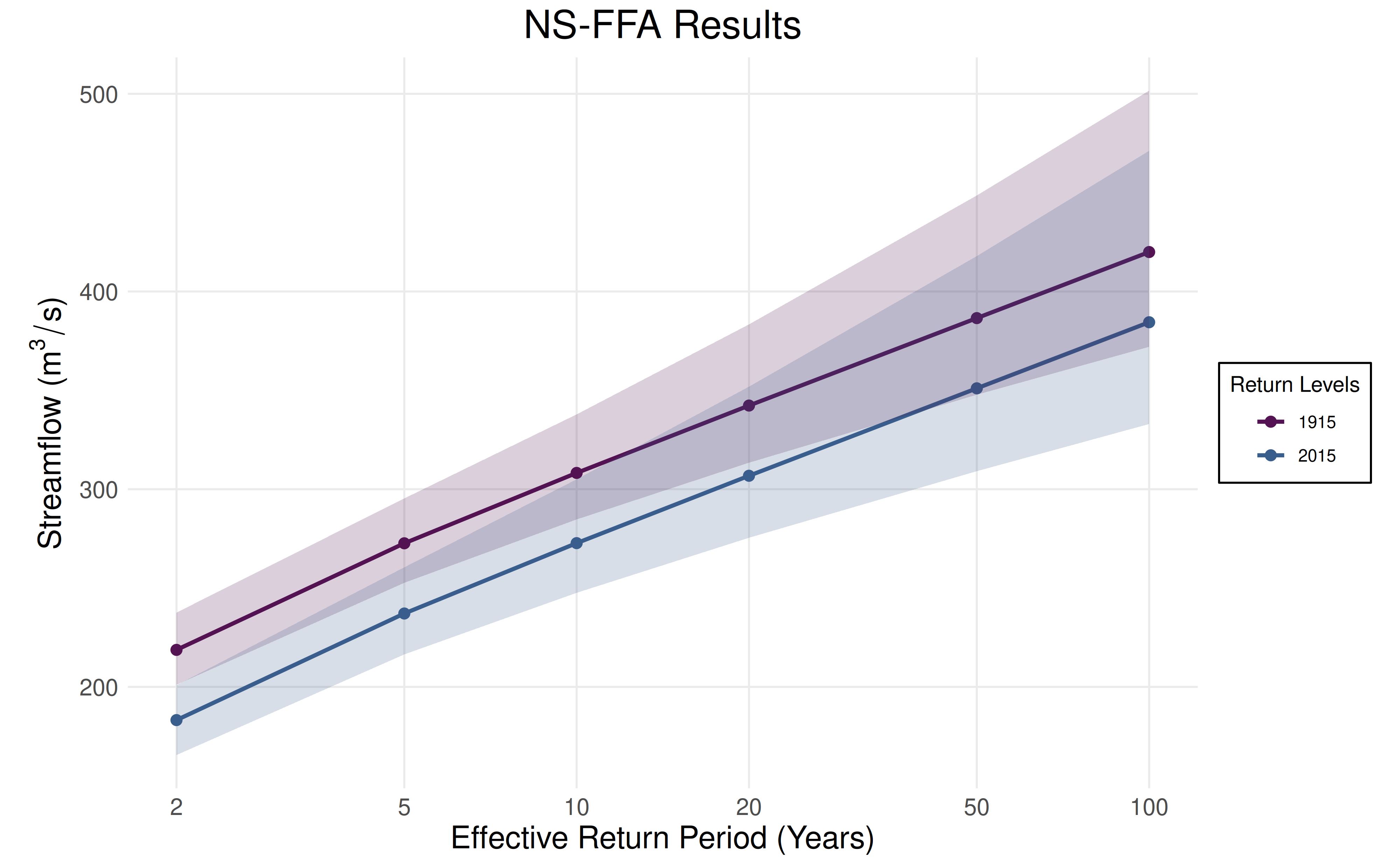
Example Conclusion: In 2025, there is a \(1/20\) exceedance probability of a flood of approximately \(300\text{m}^3/\text{s}\) or greater. The estimated return levels have decreased by approximately \(50\text{m}^3/\text{s}\) between 1925 and 2025.
Note: Under nonstationarity, the return period reflects the probability distribution for a fixed year rather than a long-run average. To clarify this difference from stationary FFA, the phrase “effective return period” is used.
Model Assessment
During S-FFA model assessment, we compare the data (or “empirical
quantiles”) with the predictions of the parametric model at the plotting
positions (the “theoretical quantiles”). Unfortunately, the same method
does not work for NS-FFA, since the method of plotting positions assumes
stationarity. However, if we normalize the data using our selected
distribution, we can remove the time-dependence and use the method of
plotting positions as in S-FFA. The model_assessment
function will make the necessary adjustments for NS-FFA automatically
provided that the ns_years and ns_structure
arguments are provided.
assessment <- model_assessment(
    df$max,
    "GNO",
    "MLE",
    ns_years = df$year,
    ns_structure = ns_structure
)

plot_nsffa_assessment(assessment)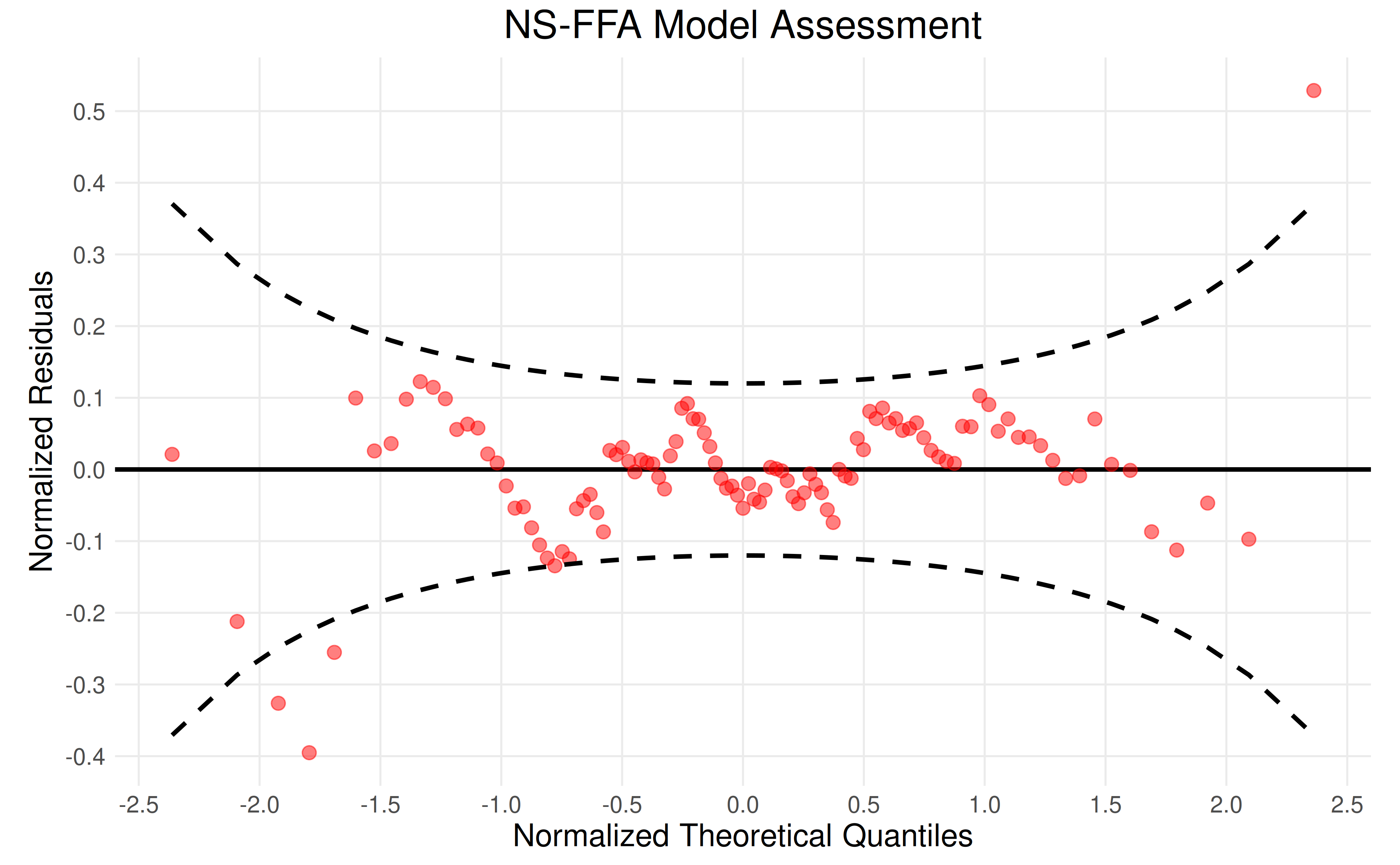
The model assessment plot shown above depicts the normalized theoretical quantiles on the x-axis and the difference between the theoretical and empirical quantiles on the y-axis. The dashed black lines are the 95% confidence bounds. From this plot, we can see that the model is a suitable fit for almost all data points.