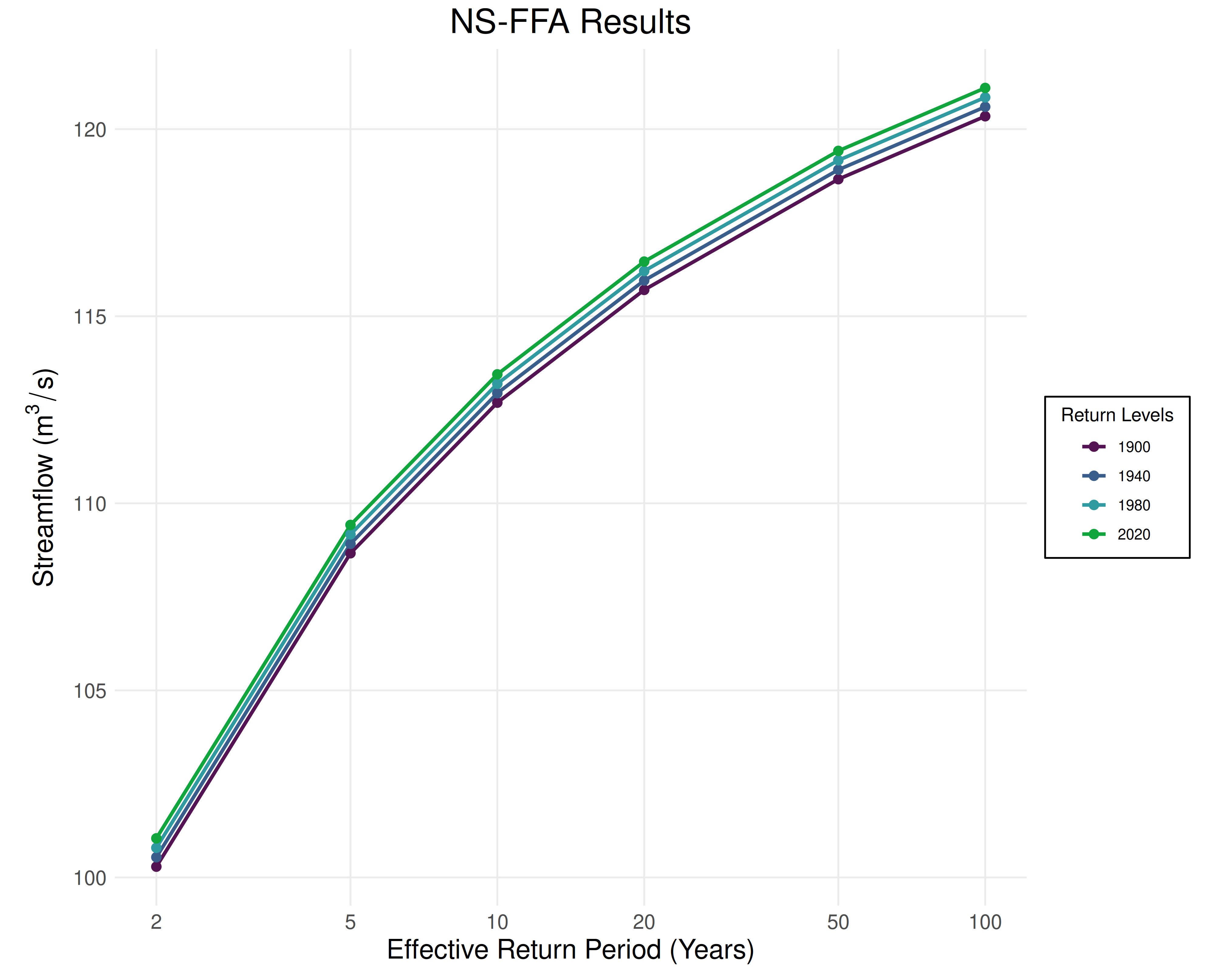
Plot Estimated Return Levels for NS-FFA — plot_nsffa

Generates a plot with effective return periods on the x-axis and effective return levels (annual maxima magnitudes) on the y-axis. Each slice is displayed in a distinct color. Confidence bounds are shown as semi-transparent ribbons, and the point estimates are overlaid as solid lines. Return periods have a logarithmic scale.

Usage

plot_nsffa_estimates(
  results,
  slices = c(1900, 1940, 1980, 2020),
  periods = c(2, 5, 10, 20, 50, 100),
  ...
)

Arguments

results: A fitted flood frequency model generated by fit_lmoments(), fit_mle() or fit_gmle() OR a fitted model with confidence intervals generated by uncertainty_bootstrap(), uncertainty_rfpl(), or uncertainty_rfgpl().
slices: Default time slices for plotting the return levels if confidence intervals are not provided.
periods: Numeric vector used to set the return periods for FFA. All entries must be greater than or equal to 1.
...: Optional named arguments: 'title', 'xlabel', and 'ylabel'.

Value

ggplot; a plot with one line and ribbon per slice.

Examples


# Fit a nonstationary model  
data <- rnorm(n = 100, mean = 100, sd = 10)
years <- seq(from = 1901, to = 2000)
ns_structure <- list(location = TRUE, scale = FALSE)

results <- fit_mle(
     data, 
     "GEV", 
     ns_years = years, 
     ns_structure = ns_structure
)

# Generate the plot
plot_nsffa_estimates(results)