Many factors can produce nonstationarity in annual maximum
series (AMS) data, including changes in climate, land use/cover, and
water management. This vignette demonstrates how to use the
ffaframework to check for evidence of nonstationarity in
the mean of a time series.
List of Tests
Mean Trend Tests
| Function | Purpose |
|---|---|
eda_mk_test |
Tests for a monotonic trend (Mann-Kendall test). |
eda_bbmk_test |
Tests for a monotonic trend under serial correlation (BBMK test). |
Stationarity Tests
| Function | Purpose |
|---|---|
eda_spearman_test |
Tests for serial correlation (Spearman test). |
eda_kpss_test |
Tests for a stochastic trend (KPSS test). |
eda_pp_test |
Tests for a deterministic trend (Phillips-Perron test). |
Variability Trend Tests
| Function | Purpose |
|---|---|
| MW-MK Test | Tests for a trend in the variability (MWMK test) |
eda_white_test |
Tests for time-dependence in the variability (White test). |
Trend Estimation (Mean & Variability)
| Function | Purpose |
|---|---|
eda_sens_trend |
Estimates slope and intercept of a linear trend (Sen’s trend estimator). |
eda_runs_test |
Evaluates residuals’ structure under linear model assumptions (runs test). |
Case Study
This vignette will explore data from the Bow River at Banff (05BB001)
hydrological monitoring station. The remoteness of this station means
that trends annual maxima are caused by changes in climate as opposed to
changes in land use or cover. Data for this station is provided as
CAN-05BB001.csv in the ffaframework
package.
library(ffaframework)

df <- data_local("CAN-05BB001.csv")
head(df)
#>   year max
#> 1 1909 314
#> 2 1910 230
#> 3 1911 264
#> 4 1912 174
#> 5 1913 232
#> 6 1914 214

plot_ams_data(df$max, df$year, title = "Bow River at Banff (05BB001)")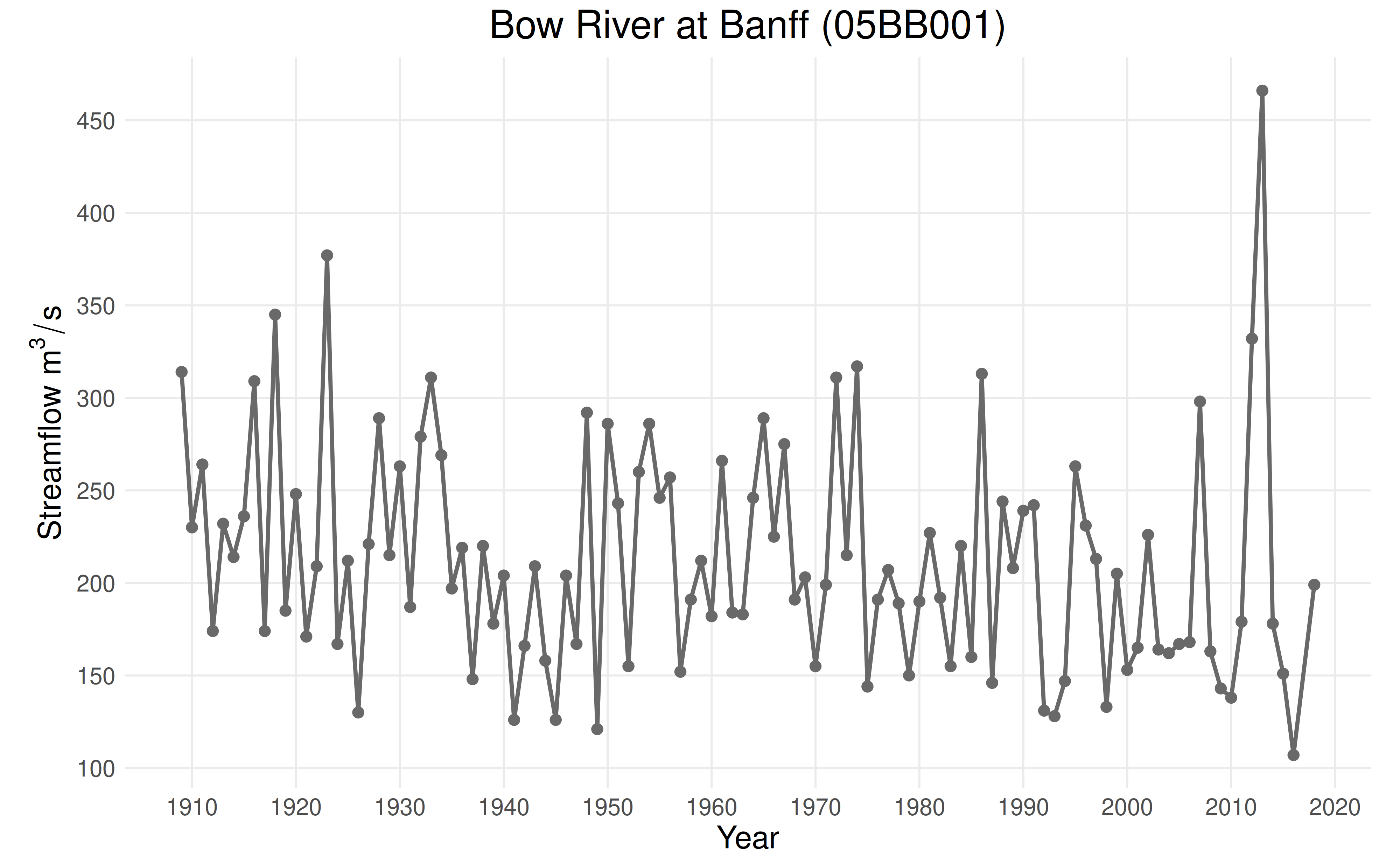
Assessing Trends in the Mean
Mann-Kendall Test
The Mann-Kendall test is a non-parametric test used to detect monotonic trends in a time series. Under the null hypothesis, there is no trend.
Pass a vector of annual maximum series (AMS) data to
eda_mk_test() to perform the Mann-Kendall test.
mk_test <- eda_mk_test(df$max)

print(mk_test$p_value)
#> [1] 0.006773098Conclusion: At a p-value of \(0.0067\), we reject the null hypothesis. There is statistical evidence of a trend in the mean.
Spearman Test
The Spearman test is used to check for serial correlation, which can cause the Mann-Kendall test to identify a spurious trend. The smallest lag at which the serial correlation is not statistically significant is known as the “least lag”.
spearman_test <- eda_spearman_test(df$max)

print(spearman_test$least_lag)
#> [1] 1

plot_spearman_test(spearman_test)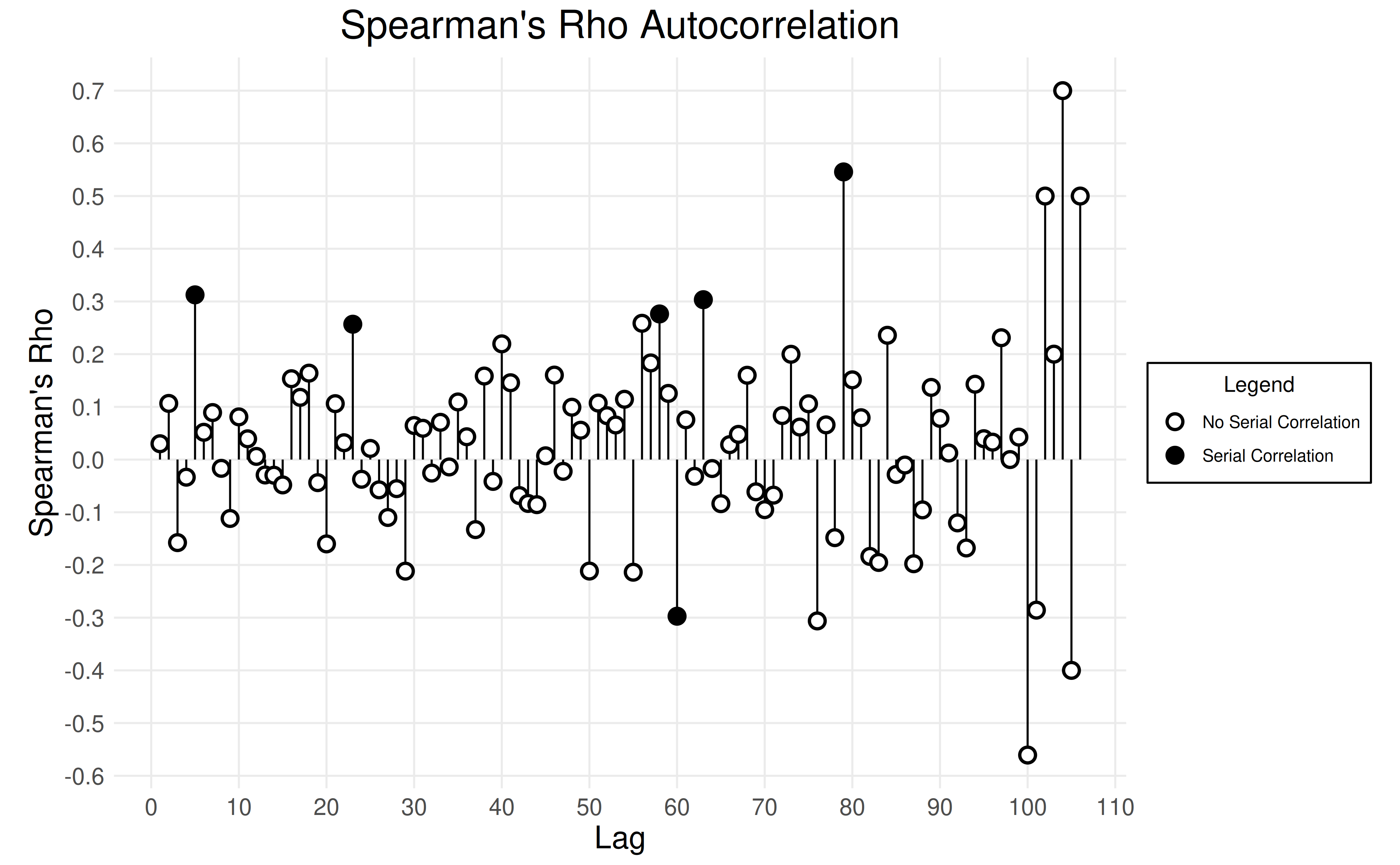
Conclusion: A least lag of 1 provides no evidence of serial correlation.
Further Tests
If the Spearman test identified serial correlation, we would use the
BBMK test (with eda_bbmk_test) to check for a monotonic
trend under serial correlation. The BBMK test uses a reshuffling
procedure to remove serial correlation from the data.
The Phillips-Perron (eda_pp_test) and KPSS
(eda_kpss_test) tests are used to check for a unit root (or
stochastic trend) in the data. A unit root is an extreme type
of serial correlation that creates unpredictable variation in the data.
Since we did not find evidence of serial correlation in the Spearman
test, it is not necessary to apply these tests. The Phillips-Perron and
KPSS tests have opposite hypotheses: the Phillips-Perron assumes the
presence of a unit root as the null hypothesis, while the KPSS test does
not.
Sen’s Trend Estimator
While the Mann-Kendall identified a significant monotonic trend, it did not estimate its slope or intercept. We can estimate the monotonic trend using Sen’s trend estimator, which uses a non-parametric approach that is robust to outliers.
eda_sens_trend() takes two arguments: the annual maximum
series and the corresponding vector of years. Then,
plot_ams_data() can be used to generate a plot of the
results. It requires the AMS data and corresponding vector of years. It
also takes an optional arguments plot_mean and
plot_variability for plotting a trend in the mean and
variability respectively.
plot_ams_data(
    df$max,
    df$year,
    plot_mean = "Trend",
    title = "Sen's Trend Estimator (AMS Mean)"
)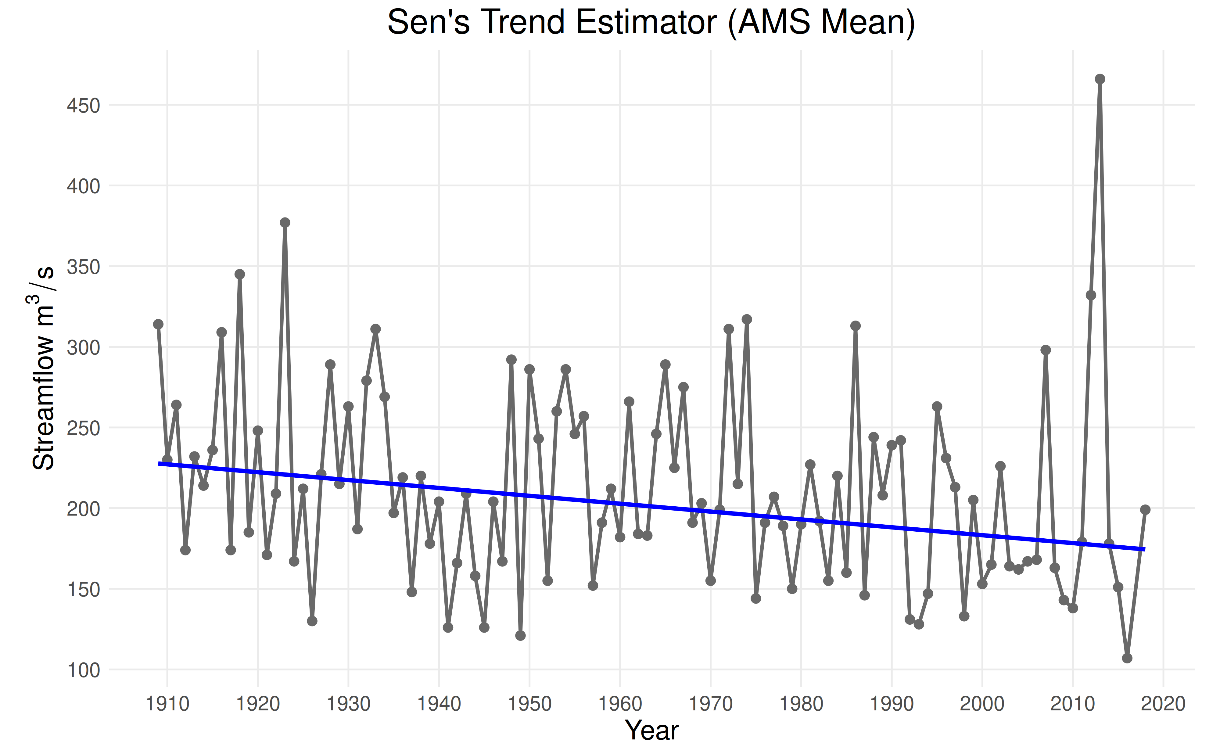
Note: The covariate is computed using the formula \((\text{years} - 1900) / 100\).
Runs Test
The previous statistical tests have assumed the nonstationarity is
linear. The runs test assess the feasibility of the linearity assumption
by checking the residuals for randomness. Alternatively,
plot_ams_data() can be used to run Sen’s trend estimator on
the data and/or variability series and then plot the results. It takes
the optional arguments plot_mean and
plot_variability in addition to the data and
years.
sens_trend <- eda_sens_trend(df$max, df$year)

runs_test <- eda_runs_test(sens_trend$residuals, df$year)

print(runs_test$p_value)
#> [1] 0.4392721

plot_runs_test(runs_test, title = "Runs Test (AMS Mean)")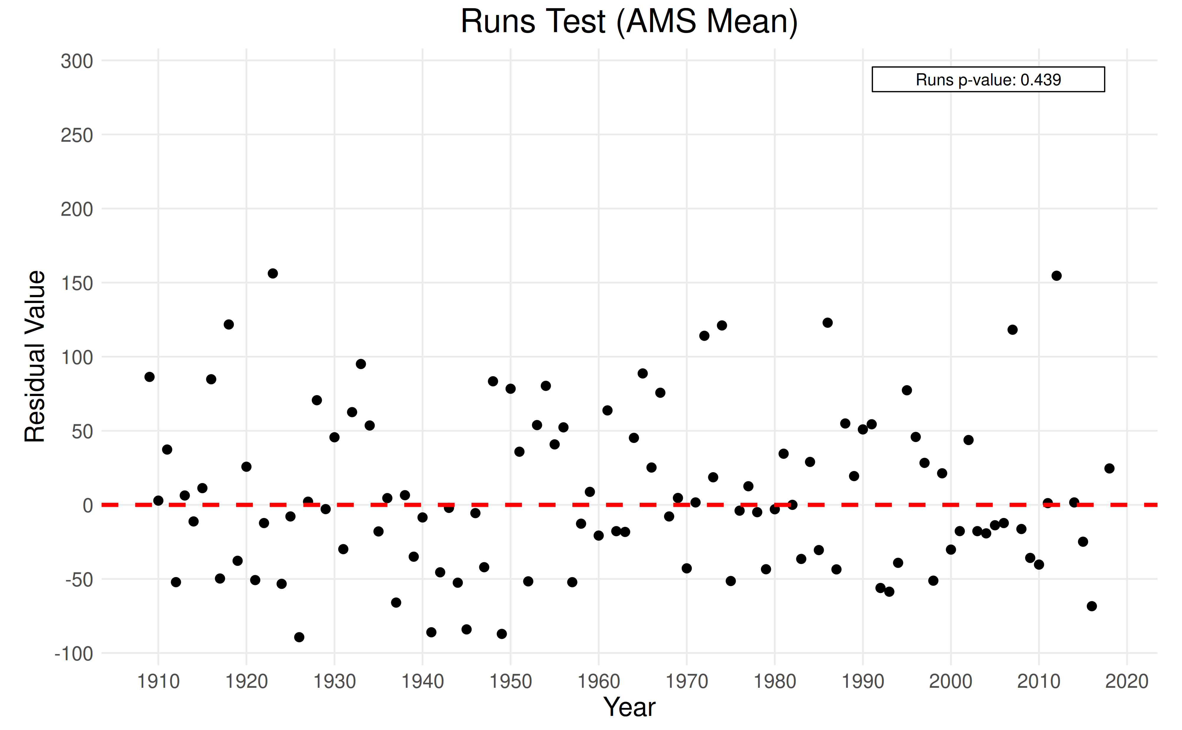
Conclusion: At a p-value of \(0.682\), there is evidence that a linear trend is suitable for the data.
Conclusion
The Mann-Kendall test identified evidence of nonstationarity in the mean of the AMS. The Spearman test did not find evidence of serial correlation, validating the results of the Mann-Kendall test. The runs test found that a linear model is suitable for the nonstationarity. Flood frequency analysis of this dataset requires a time-dependent probability model.
Recommendation: Use NS-FFA.