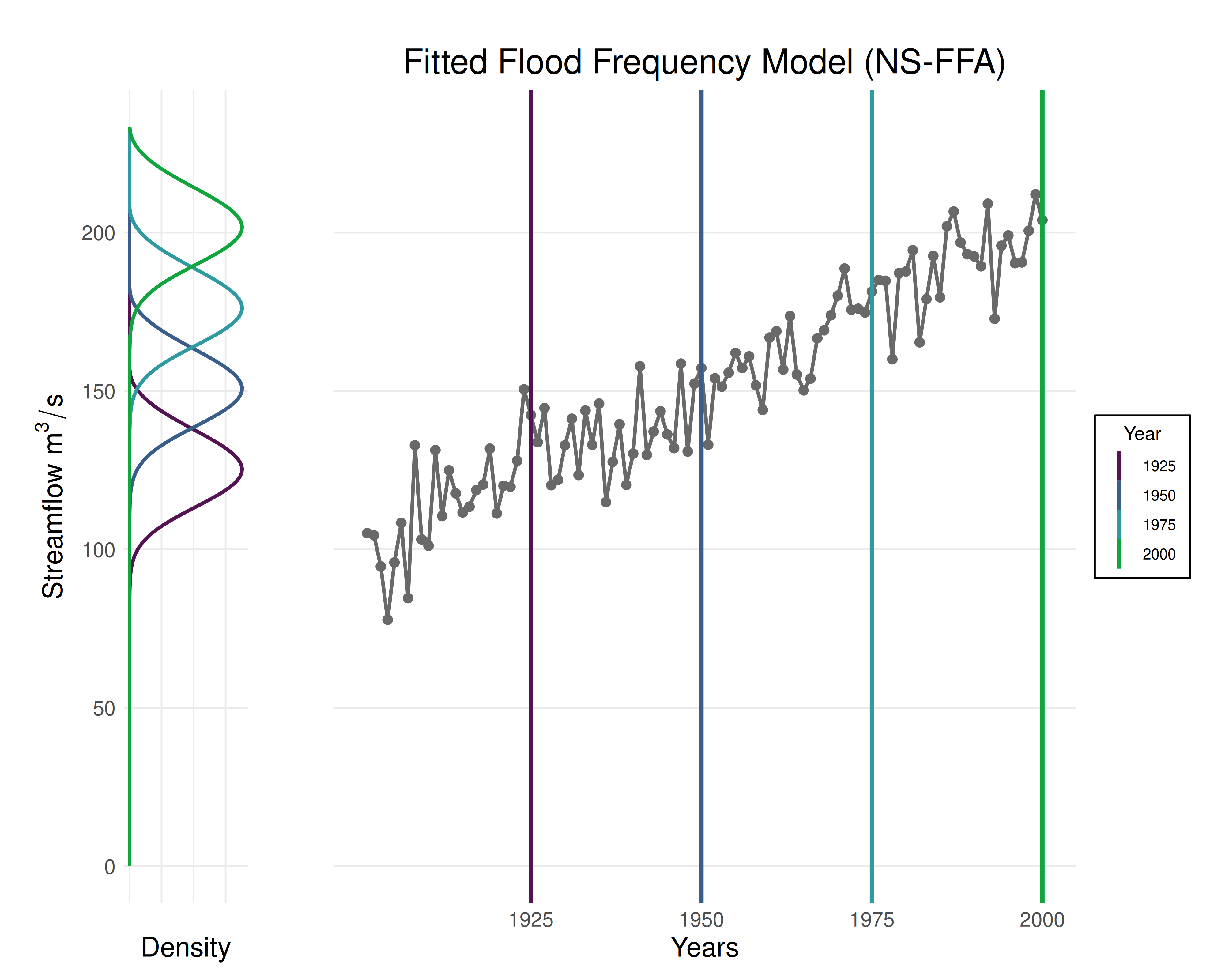
Generates a plot showing probability densities of a nonstationary model for selected time slices (left panel) and the data (right panel).
Usage
plot_nsffa_fit(
  results,
  slices = c(1925, 1950, 1975, 2000),
  show_line = TRUE,
  ...
)
Arguments
- results
A fitted flood frequency model generated by
fit_lmoments(),fit_mle()orfit_gmle().- slices
Years at which to plot the nonstationary probability model.
- show_line
If
TRUE(default), draw a fitted line through the data.- ...
Optional named arguments: 'title', 'xlabel', and 'ylabel'.