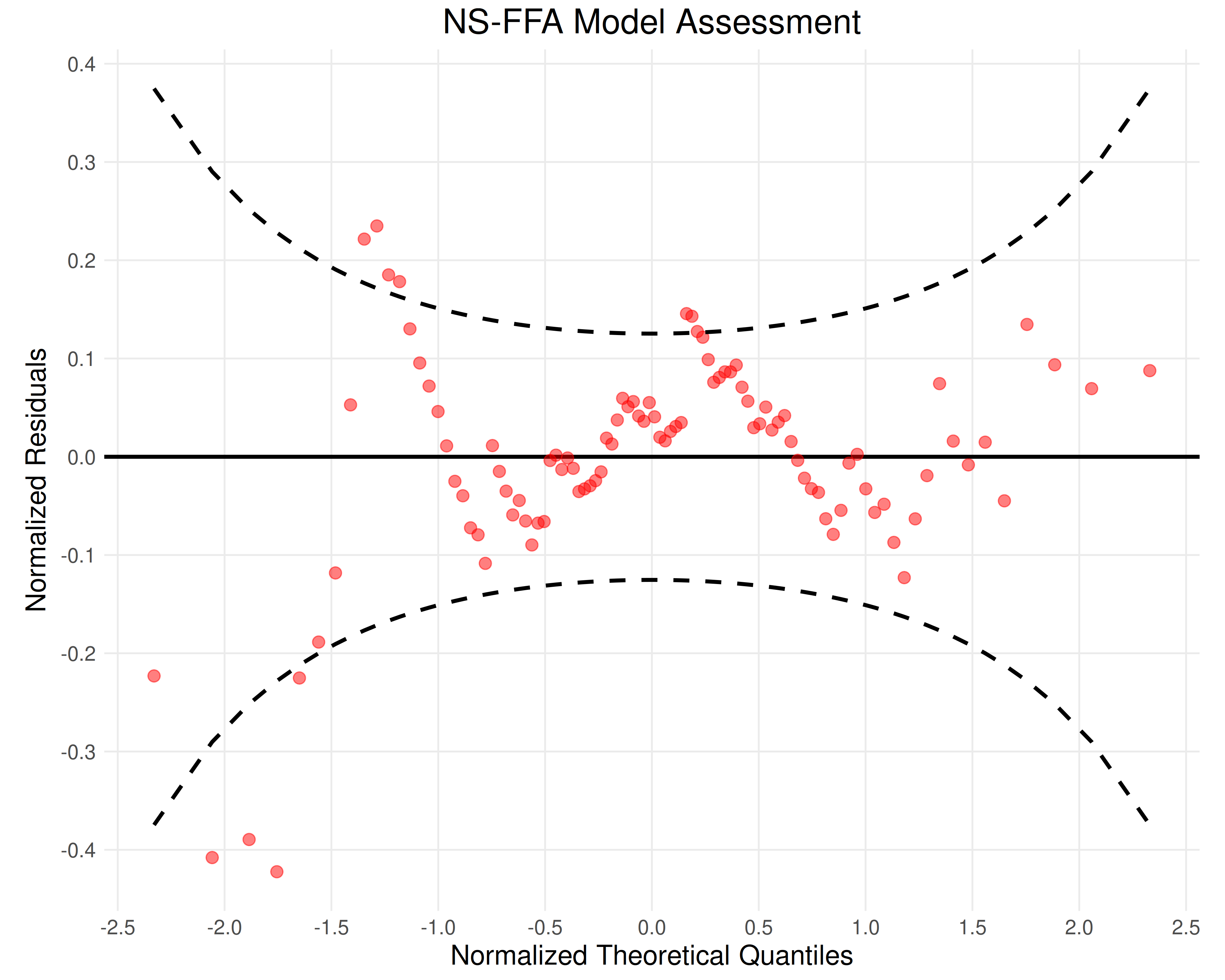
Creates a normalized and detrended quantile–quantile plot (a worm plot) comparing empirical annual maximum series data to quantile estimates from a fitted, parametric, and nonstationary model. Confidence intervals are also provided. The worm plot can be interpreted using the following heuristics:
For a satisfactory fit, the worm (red data points) should be within the 95% confidence interval (dashed black lines).
If the worm (red points) is passes above/below the origin, the model mean is too small/large respectively.
If the worm has a clear positive/negative slope, the model variance is too small/large respectively.
If the worm has a U-shape or inverted U-shape, the model is too skew to the left/right respectively.
Arguments
- results
List; model assessment results generated by
model_assessment().- ...
Optional named arguments: 'title', 'xlabel', and 'ylabel'.
Value
ggplot; a plot containing:
A black line representing a model with no deviation from the empirical quantiles.
Red points denoting the estimated quantiles against the empirical quantiles.
A dashed black line showing the 95% confidence intervals of the residuals.
References
van Buuren, S., Fredriks, M. Worm plot: a simple diagnostic device for modelling growth reference curves. Statistics in Medicine 20 (8), 1259-1277. doi:10.1002/sim.746
Examples
# Initialize example data and params
data <- rnorm(n = 100, mean = 100, sd = 10) + seq(from = 1, to = 100)
years <- seq(from = 1901, to = 2000)
structure <- list(location = TRUE, scale = FALSE)

# Evaluate model diagnostics
results <- model_assessment(data, "NOR", "MLE", NULL, years, structure)

# Generate a model assessment plot
plot_nsffa_assessment(results)